ncRNA Genes @ RNAcentral
Gathering transcripts into genes
RNAcentral is a database of non-coding RNA transcripts. It contains as many of the ncRNAs as we can find that have been sequenced at some point and uploaded into something like ENA. Lots of these transcripts have been seen several times, and some of them have been seen with slight variations. Many databases provide coordinates showing where their transcripts map onto a genome, and we see that sometimes a lot of them overlap. If we see loads of transcripts piling up in one place, could it be that we are seeing a gene in that location, maybe with some noise or slplicing variability?
Creating genes has been an ambition at RNAcentral for a long time, since most of the higher level annotations we want to use or make would only really make sense at a gene level. For example the Gene Ontology consortium annotates the function of genes using the GO ontology (among other things, but this is the most relevant thing they do to the point I’m making here). Those functions are annotated at the gene level for proteins, but until recently were annotated at the transcript level for ncRNAs. We know there are ncRNAs that have well-defined functions (e.g. XIST) and are real genes, but the annotations imported at RNAcentral will still end up mapped to a particular transcript, rather than the gene as a whole.
Normally, genes are called by expert interrogation of the data. Groups like GENCODE will gather the evidence for a given locus and use it to determine exactly where in the genome the start of a gene is, and what all the intron/exon structure looks like and everything else. However, ncRNA has much less curator time than protein, so this isn’t an option for us.
- The Problem: RNAcentral was historically transcript-based, but higher-level functional annotations (like Gene Ontology) make the most sense at the gene level. We don’t have the curator bandwidth to call genes manually.
- The Pipeline: We run a two-step automated pipeline:
- Pairwise transcript classification using a Random Forest model based on distance, overlap, and Sequence Ontology similarity (embedded via
node2vec). - Graph clustering using the Louvain community detection algorithm to group transcripts into genes.
- Pairwise transcript classification using a Random Forest model based on distance, overlap, and Sequence Ontology similarity (embedded via
- Naming & Metadata: Genes get stable identifiers (
RNACG...) based on a SHA256 hash of genomic coordinates, and metadata is assigned using a weighted voting system from expert databases. - The Scale: Generated 103,814 human genes from ~600,000 transcripts. On average, we map to 1.6 Ensembl genes (meaning we tend to merge what Ensembl separates).
- Limitations: Complex splicing structures (like XIST) get split, and intronic “inside-out” genes (like SNHG1) get misgrouped.
Genes from transcripts
If you go look at a random page on RNAcentral, you will probably see a genome browser display something like this one:
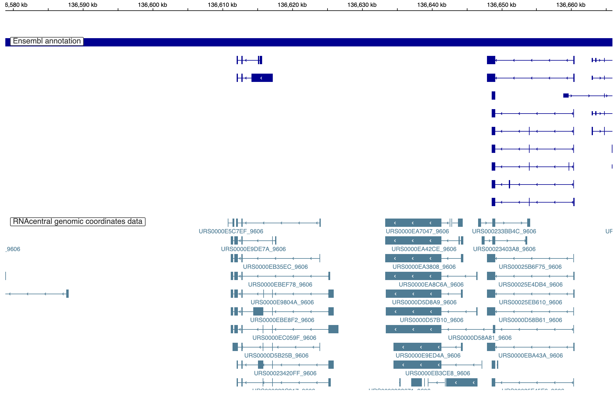
Here you can see a track showing the ensembl genome (dark blue at the top) and transcripts mapped in RNAcentral (at the bottom). When I looked at this, I noticed a couple of things:
- The ensembl annotations don’t always match up with mapped transcripts
- A lot of transcripts line up really well
Building on some work that was done by the RNAcentral consortium, we started to design what an ML model might look like that could coalesce these transcripts down into genes.
Model requirements
We had a set of fairly hard requirements for the model/system:
- Work using transcripts and only the data we have available after mapping them onto a genome. Try not to require ‘higher level’ data like expression or anything
- Work across all organisms. Human genes are the remit of HGNC and Gencode, but there aren’t groups calling genes for non model organisms like cows
- Be fast enough to run within the RNAcentral release pipeline
- Produce somewhat stable genes with somewhat stable identifiers
Architecture choice
I decided to go with a simple classic ML architecture, Random Forests. These are quite robust to overfitting and work really well on small tabular datasets, which is sort of what we have. They also allow looking at the feature importance to see if the decisions taken by the model make biological sense, based on what the features being used are.
Random forests take a vector of features and output a classification. The way I decided to map this onto the transcript coalescense problem was a pairwise classification - are these two transcripts part of the same gene or not? We can make some traning data for this using the ensembl annotations we do have (which group transcripts to a gene already). Negative samples come from nearby genes whose transcripts should not be grouped. I defined nearby as 1000 nucleotides, which I’ve been told is really not far at all in genomics.
Making the problem into a binary classification simplifies the curation of a training set, and makes the evaluation of this bit of the modelling quite straightforward. It does however mean that I had to do some feature engineering
Features - Distance vs Overlap
When I worked in radiotherapy, one of my colleagues had a (well founded) hatred of overlap metrics for assessing image segmentation quality. Basically, overlaps don’t work very well when one thing is much smaller than the other (it’s either close to zero of 100% depending which way round you look), and they are sensitive to the volume of the things being compared (99% overlap of a big thing is less impressive than 99% overlap of a small thing).
The preferred method was to calculate distance to agreement, or one of the variants of it. In radiotherapy this meant doing a calculation in 3D space between two surfaces defined by a set of points lying on the edge of a segmentation. That’s a relatively involved calculation, but it gives a more realistic picture of what’s going on, so its worth it.
However, when looking to calculate features for grouping transcripts into genes, we only have one dimension, so each of these feature classes are about the same level of difficulty. Therefore, I calculated both and let the model select which was the morre informative.
Looking at old work from consortium meetings I decided on the following features:
- 5’ exon overlap. A number in the range 0-1, can be assymetric
- Number of exons having >0.9 overlap.
- Distance to agreement between 5’ exon starts. This is a number that’s essentially unbounded, but probably less than 1000 given the selection criteria.
- Distance to agreement of the 3’ end of the 5’ exon. Again, essentially unbounded, but this came from looking at where consortium members had drawn vertical lines on a printout of the genome browser - it wasn’t complete guesswork.
All these features can be calculated from just the coordinates on the genome, which is ideal. But, it is missing a potentially large problem - what if we have two dissimilar RNA types close together? At the moment the model might group them together in a way that doesn’t make sense.
Features - RNA type
RNAcentral provides a Sequence Ontology type ID for every transcript. The SO allows a precise definition of the type of an RNA by providing an ID something like SO:0001877 (lncRNA). I needed a way to turn two SO IDs into a number that quantifies how similar they are.
This turned into a bit of a sidequest. The SO is a directed acyclic graph, meaning each node has an is_a relationship with other nodes. For example SO:0001877 (lncRNA) has an is_a relationship to SO:0000655 (ncRNA). I used the graph nature of the SO to tran a Node2Vec model on SO IDs. This makes random walks in the graph, following its connections properly, and then does a Word2Vec style embedding on the resulting lists of terms. In this way, terms that are close together in the graph should end up embedded into vectors that are close together in embedding space. I think it might also do other stuff that you get with Word2Vec, like allow some funky vector arithmetic, but I didn’t use that - I just wanted the cosine similarity of two SO terms so I sould feed it into the Random Forest model.
It worked fairly well. For example two things that shoould be close SO:0001877 (lncRNA) and SO:0001463 (lincRNA) have a cosine similarity of 0.70, while things that should not be similar like SO:0001877 and SO:0000407 (cytosolic_18S_rRNA) had a lower similarity of 0.43. I learned some stuff about this that mighe change in a future version, but I’ll talk about that later.
Random Forest performance
So, I now have my feature set and I can start to train some stuff. I trained the model of pairwise feature calculations of randomly shuffled ensembl genes for human. The dataset is split after calculating features into a train, val and test. I’m pretty sure there’s no data leakage possible so this is done randomly, and therefore it is possible that pairs of transcripts from the same gene ended up in the train and test sets (i.e if a gene has three transcripts A, B and C, A vs B could be in the train set and A vs C inthe test set - I think this is fine).
The models were trained in the usual 5-fold cross validation style, and evaluated on the held out test set. I also prepared a feature set from genes for mice, also from ensembl. The RF model was almost perfect.
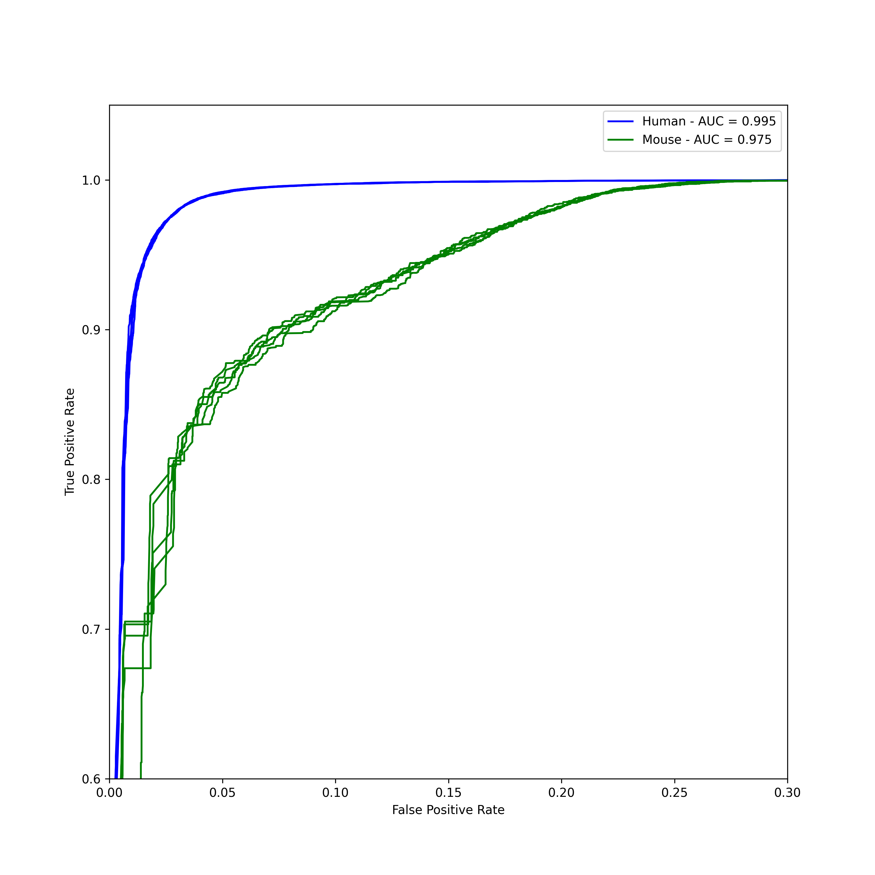
This plot is risky, because it makes the mouse result look rubbish - while in fact an average ROC of 0.975 is still fantasitc. The plot is zoomed right in to show any difference.
At this point then, I have a model that is really good at telling whether two transcripts came from the same gene. This is the first step, but it isn’t the end goal of a gene predicting model.
Genes from Graphs
To make a single gene from a collection of pairwise gene membership predictions, I needed to put the transcripts into a graph. Putting transcripts in a graph means modeling each transcript as a node, and creating edges where the random forest predicts they are members of the same gene. I do this for chunks of the chomosome, rather than the whole thing, to prevent it blowing up the memory.
Once the graph is built, we have a few choices for how to create genes. The simplest was to just to do a connected component analysis on the nodes and edges, which was my first pass solution, but it was suggested that using the Louvain community detection algorithm (with probabilities as an edge weights) might work better.
The Louvain method works bottom-up to shuffle nodes in the graph into communities that maximize the modularity of the graph. It starts locally with the real nodes, and progresses to larger scales by treating low-level communities as supernodes in a condensed graph, and trying to determine their community layout as well. In this way, local-scale graph structure can be aggregated with longer range interactions to build genes over long distances.
The Louvain method is what we used in the final version, and it does a pretty good job.
What the Random Forest Cared About (Feature Importance)
Once the model was trained, I wanted to see what it was actually using to make its decisions. Looking at the feature importances (which would be Fig 4 in the paper), the results made a lot of biological sense: * The absolute winner: The distance between the 5’ coordinates of the transcripts. If the 5’ starts are close together, they are very likely to be part of the same gene. * Runner up: Strand compatibility (transcripts must be on the same strand, obviously). * The surprise: Sequence Ontology (SO) type similarity was much less important than I expected. In hindsight, this is probably because the training data (drawn from Ensembl’s known genes) had relatively low diversity in RNA types, so the model didn’t need to rely on the node2vec embeddings as much.
Stable Identifiers and Naming (or, how not to break user links)
One of our hardest requirements was making sure that when we release a new version of RNAcentral, we don’t break everyone’s links by completely renaming the genes.
We settled on a naming pattern: RNACG<species-prefix><11-digit hash >.<version>
For human genes, there is no species prefix (e.g. RNACG0000012345.1). The 11-digit hash is computed using a SHA256 hash of the gene’s coordinates, chromosome, and assembly ID. The version number starts at 1, and only increments if the transcripts within the gene change (like when transcripts are added or removed, or the start/end coordinates shift). If nothing changes between database releases, the identifier stays exactly the same.
Assigning Metadata (Weighted Voting)
Once we’ve grouped a bunch of transcripts into a gene, we need to decide what to call it and what RNA type it is. Transcripts in RNAcentral come from 52 different expert databases, and they don’t always agree.
To solve this, I built a weighted voting system. Annotations from curated, high-confidence databases (like HGNC, FlyBase, and GENCODE) are given more weight than raw sequence submissions (like ENA). For Rfam and R2DT structural annotations, we only count their “votes” if the family matches over 90% of the longest transcript in the gene. This keeps the metadata clean and prevents a single noisy transcript from mislabeling the entire gene.
The Numbers & Real-World Quirks
When we ran this on the human genome, the model grouped 600,225 transcripts into 103,814 human genes spanning 56 different SO types. By far the most common genes were: * Long non-coding RNAs (lncRNAs): 65,187 genes * Antisense lncRNAs: 16,790 genes * Pre-miRNAs: 8,560 genes
An average ncRNA gene in RNAcentral contains about 6 transcripts, though this ranges from a minimum of 2 up to a massive 4,001 transcripts for mitochondrial SSU rRNAs (which have tons of sequenced fragments in the database).
Comparing our predicted genes to Ensembl, we found that on average, an RNAcentral gene maps to 1.6 Ensembl genes. This means our pipeline is slightly “lumpier” than Ensembl—it tends to merge things that Ensembl considers separate.
The Good, the Bad, and the XIST
We looked at some well-known case studies to see how the model performed in the real world: * The Successes: High-profile lncRNAs like MALAT1 and NEAT1 clustered perfectly into single, neat gene entries. * The Splicing Trap: XIST (the famous X-inactive specific transcript) was split across five separate genes in our database. XIST has a highly complex alternative splicing structure with huge genomic distances between its alternative 5’ exons. Because our model relies heavily on 5’ start proximity, it assumed these transcripts belonged to different genes. In general, complex lncRNAs with highly variable splicing are the pipeline’s biggest weakness.
Limitations & Future Directions
The current model represents a “superset” of ncRNA genes—meaning it has very high recall but relatively low precision. We’d rather group a few separate genes together than miss a real gene locus entirely, but there is still plenty of room for improvement:
- Intronic “Inside-Out” Genes: Genes like SNHG1 host small nucleolar RNAs (snoRNAs) inside their introns. Our model struggles with these because Ensembl’s training data doesn’t split intronic ncRNAs out, so the Random Forest hasn’t learned how to separate them.
- Evolutionary Filtering: We are working on using sequence homology to filter out predicted genes that show no signs of evolutionary conservation. If a predicted gene isn’t conserved across related species, it’s likely just noise.
- Protein-Coding Filtering: In future releases, we plan to implement additional QA steps (using Pfam, stopFree, and tcode) to filter out transcripts with high protein-coding potential, ensuring our ncRNA database stays strictly non-coding.